Transformers, From First Principles

Motivation

This writing is my reflection from CS312: Natural Language Processing. During the transformer architecture unit, the overall flow was not immediately clear to me, so I looked for a more grounded way to rebuild the architecture from first principles. I came across Stanford CME295: Transformers and Large Language Models and Neel Nanda’s Transformer walkthrough series. Both helped me rebuild the architecture from scratch in a way that actually made sense to me.

What follows is my attempt to reconstruct the transformer from the ground up, the way I wish it had been explained the first time. I work primarily from Neel Nanda’s clean implementation of GPT-2, because I believe the only honest way to understand an architecture is to build it yourself, layer by layer, and verify each piece against a reference model.

What is a Transformer?

Transformers exist to model text. The core task is deceptively simple: given a sequence of tokens, predict the next one. Repeat that autoregressively and you get a language model that generates coherent text. What makes this work at scale is a training trick worth appreciating: when you feed a model 100 tokens, it does not produce one prediction. It produces 100 predictions, one per position. Because of causal attention, the prediction at position 50 only sees tokens 1 through 50, never anything ahead. This means a single forward pass gives you 100 gradient signals instead of one, which makes training dramatically more efficient.

At the structural level, a transformer runs the same computation in parallel at every sequence position, uses attention to move information between positions, and can in principle handle sequences of arbitrary length, with some practical limits we will get to.

Inputs & Outputs

The input to a transformer is a sequence of integers, token IDs. The output is a tensor of logits with shape [batch, position, d_vocab]. For each position in the input sequence, the model produces a vector of size equal to the vocabulary, where each entry scores how likely that token is to come next.

Converting these raw logits into a probability distribution requires a softmax. The exponential makes every value positive, and dividing by the sum normalizes them to add to one. To generate text, you take the logit vector at the last position, apply softmax, sample or take the argmax, append that token to the input, and run the model again. This is autoregressive generation.

Tokens

Language is not naturally numerical. To feed text into a neural network, we need a way to convert it to integers. The standard approach is a vocabulary of tokens, subword units learned from data.

GPT-2 uses Byte-Pair Encoding (BPE). The algorithm starts with the 256 ASCII characters as base tokens, finds the most common adjacent pair, merges them into a new token, and repeats 50,000 times. This gives a vocabulary that balances coverage with efficiency: it can represent any text while giving common words and subwords their own compact units.

One important nuance is that whether a word starts with a space or a capital letter changes which token it maps to. The tokenizer treats "Ralph" and " Ralph" as entirely different sequences. Arithmetic is even messier because numbers bundle in unpredictable ways depending on how common they are in the training corpus. Tokenization is a genuine headache, and it is worth staying aware of its quirks throughout any NLP work.

Once we have integers, we convert them to vectors with an embedding lookup table of shape [d_vocab, d_model]. Each token ID indexes one row of this matrix. The result is a sequence of dense vectors, one per token, each of dimension d_model, which is 768 in GPT-2 small.

Logits & Generation

After all the transformer layers have processed the token embeddings, a final unembedding step projects each position’s residual stream vector back up to vocabulary size. These are the logits. To generate the next token:

1. Convert text to tokens.
2. Run the model to get logits of shape [batch, position, d_vocab].
3. Take the logit vector at the last position and apply softmax.
4. Sample or take the argmax to get the next token.
5. Append to the input and repeat.

This loop is autoregressive generation. Each call to the model adds one token, but because the full context is re-processed each time, the model can condition on everything that came before.

Architecture

GPT-2 small has the following shape:

Parameter	Value	Meaning
d_model	768	Residual stream dimension
n_layers	12	Number of transformer blocks
n_heads	12	Attention heads per block
d_head	64	Dimension per head (d_model / n_heads)
d_mlp	3072	MLP hidden dimension (4 × d_model)
n_ctx	1024	Maximum context length
d_vocab	50257	Vocabulary size

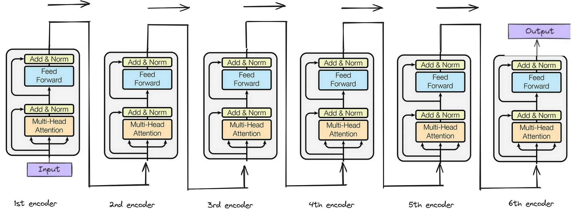
The high-level flow is token embeddings plus positional embeddings feeding into a residual stream, which then passes through 12 transformer blocks. Each block contains a LayerNorm, an attention sublayer, another LayerNorm, and an MLP sublayer. A final LayerNorm and unembedding step produce the output logits.

One useful clarification is that when people say a transformer has k layers, they usually mean k blocks, where each block contains both an attention layer and an MLP layer. GPT-2 small has 12 blocks and 24 total sublayers.

Attention

Attention is the only part of a transformer that moves information between sequence positions. Everything else, including embeddings, MLPs, and LayerNorm, operates independently at each position.

Each attention layer contains n_heads heads that act independently and additively. Their outputs are summed and added back to the residual stream. Each head does two conceptually separate things.

• Pattern: it computes an attention distribution over all prior positions, deciding where to read from.
• Move: it uses that distribution to aggregate values from source tokens into a weighted mix and project that mix back into model space.

The key insight for me was that figuring out which tokens to attend to is separate from figuring out what information to copy from them. Queries and keys handle the first. Values and the output matrix handle the second. Keeping these separate makes attention much easier to understand.

In self-attention, the query, key, and value vectors are all computed from the same sequence, but they play different roles. A query represents what the current position is looking for. A key represents what each position offers as something to be matched against. A value represents the information that actually gets moved if a position is attended to.

This differs from encoder-decoder attention, where the decoder attends to hidden states produced by a separate encoder. The dot-product mechanism is similar, but the source of the keys and values is different.

Parameter shapes per layer, GPT-2 small

Parameter	Shape	Concrete GPT-2 small shape
W_Q, W_K, W_V	[n_heads, d_model, d_head]	[12, 768, 64]
W_O	[n_heads, d_head, d_model]	[12, 64, 768]
b_Q, b_K, b_V	[n_heads, d_head]	[12, 64]
b_O	[d_model]	[768]

MLP Layers

After each attention sublayer, a two-layer MLP processes every position independently. The structure is a linear projection up to d_mlp = 4 × d_model, followed by a GELU activation, followed by a linear projection back down to d_model.

Once attention has routed relevant information to a given position, the MLP performs position-wise computation: feature detection, transformation, and nonlinear mixing. The widening to 4x gives the network room to represent many features before compressing them back.

Residual Stream

The residual stream is the central object of a transformer. At every position in the sequence there is a vector of dimension d_model that starts as the token embedding, gets updated additively by each attention and MLP sublayer, and ends as the input to the unembedding.

The critical word is additively. Neither attention nor the MLP replaces the residual stream. They each add their output to it, so every layer has direct read and write access to a shared memory space.

That shared space is what makes composition possible across layers. One head can build on the output of another simply because both are reading from and writing to the same running representation.

LayerNorm

LayerNorm is applied at the start of each sublayer and before the final unembedding. It normalizes each residual stream vector independently by subtracting the mean, dividing by the standard deviation, and then applying a learned elementwise scale and bias.

In practice, LayerNorm is almost linear but not quite. That makes it both useful and slightly annoying for interpretation, because changes in one dimension can affect the normalization of the whole vector.

Positional Embeddings

Attention by itself is position-agnostic. Without positional information, the model has no built-in sense of order or distance. GPT-2 solves this using learned absolute positional embeddings.

Transformers process tokens in parallel rather than step by step like an RNN, so they do not get order for free. Positional embeddings put order back into the input: they tell the model what token is present and where that token sits.

These are vectors of shape [n_ctx, d_model] that are added to the token embeddings before the first transformer block. The model therefore learns which positional information is useful rather than having it hard-coded.

Masked Attention in the Decoder

In decoder-only and decoder-side transformer blocks, attention is usually masked. The mask prevents a token from attending to future tokens. During training, the model may receive the whole sequence at once, but the prediction at position 5 should not be allowed to peek at position 6. Otherwise, the next-token prediction task would become a leak rather than a learning problem.

The causal mask enforces the same constraint the model will face during generation. Each position can use the tokens before it, and sometimes itself depending on implementation, but not the tokens after it. This is what keeps generation autoregressive while still allowing training to be parallelized across positions.

Putting it Together

The full forward pass of a GPT-2 style transformer looks like this:

The architecture is modular: attention moves information between positions, MLPs transform each position, and the residual stream ties the pieces into one coherent computation.

When I finally built this from scratch in PyTorch and checked each piece against GPT-2, the architecture stopped feeling like a black box. That was the feeling I was chasing.