
Motivation
When I first looked at speech processing, I thought of it as a simple conversion problem: audio in, text out. But that feels too narrow. Speech is not just language stored inside sound. It is a physical signal shaped by the speaker, the room, the microphone, background noise, accent, emotion, and the timing of conversation.
That is part of what makes speech processing different from ordinary text NLP. With text, the model starts with discrete symbols. With speech, it has to make sense of the signal itself first. It has to turn vibration into numbers, numbers into patterns, patterns into linguistic units, and linguistic units into meaning.
This note follows that path: what speech processing is, why speech is hard, how computers “hear,” then ASR, and finally speech translation.
What is Speech Processing?
Speech processing is the field that allows computers to analyze, understand, and generate human speech. A system may listen to a voice recording and produce a transcript. It may detect who is speaking, clean noisy audio, translate speech into another language, or generate a spoken response.
In the simplest form:
speech processing turns sound into something useful.
That useful thing may be text, but it does not have to be. It can also be a speaker label, an intent, a command, a translated subtitle, a synthetic voice, or a response from an audio assistant.
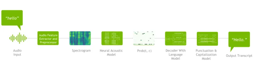
Figure 1. A high-level speech processing pipeline. Human speech is captured as audio, converted into digital representations, processed by a model, and finally turned into text, action, translation, or speech.
The important point is that speech processing sits between several fields at once. It needs signal processing because speech starts as a physical wave. It needs linguistics because the signal carries language. It needs machine learning because modern systems learn from large audio datasets. And it needs NLP because many downstream tasks eventually depend on language understanding.
Why Speech Is Hard
Speech is easy for humans partly because we are good at repairing missing information. We can understand someone in a noisy café, guess a word from context, adjust to an unfamiliar accent, and ignore background noise without thinking too much.
A computer does not get that ability for free. The same sentence can look very different as an audio signal depending on who says it, how fast they speak, how close they are to the microphone, whether the room has echo, and whether other sounds happen at the same time.
This means the model is not only learning words. It is learning to separate the linguistic content from everything else that changes the surface signal. It has to infer which parts of the audio correspond to speech, which parts come from the speaker’s identity or emotion, and which parts come from the environment.
A useful mental model is:
Speech = Language + Speaker + Environment + Interaction
The language tells us what was said. The speaker tells us who said it and how they said it. The environment tells us what kind of acoustic world the speech happened in. The interaction tells us what the utterance is trying to do.
That is why speech processing is broader than “speech-to-text.” Speech-to-text is only one part of the story.
Core Domains in Speech Processing
The first major domain is recognition and understanding. This is where automatic speech recognition belongs. The system tries to answer questions like: what was said, what does it mean, and who said which part? This includes ASR, spoken language understanding, keyword spotting, speech translation, conversational speech recognition, and speaker-attributed ASR.
The second domain is speaker and paralinguistic analysis. Here, the model is not only interested in words. It may care about who is speaking, whether two recordings come from the same speaker, what emotional state is expressed, or which person is actively speaking in a video. Speaker diarization is a good example: instead of giving one long transcript, the system separates the conversation into different speakers.
The third domain is acoustic scene and speech enhancement. Real audio is rarely clean. A model may need to suppress background noise, separate overlapping speakers, remove reverberation, or detect non-speech events in the environment. This is important because a system that works in a studio recording may fail in a classroom, street, meeting room, or video call.
The fourth domain is speech generation and conversion. Text-to-speech turns written text into spoken audio. Voice conversion changes one voice into another. Speech-to-speech translation takes speech in one language and outputs speech in another. Speech editing modifies spoken audio while trying to preserve naturalness.
So the field is not one task. It is a collection of problems around sound, language, speaker identity, and interaction.
How Computers “Hear”
A computer cannot directly hear sound the way humans do. Sound begins as continuous vibration in the air. A microphone captures that vibration and turns it into an electrical signal. Then the computer converts that signal into numbers.
The most direct representation is the waveform.
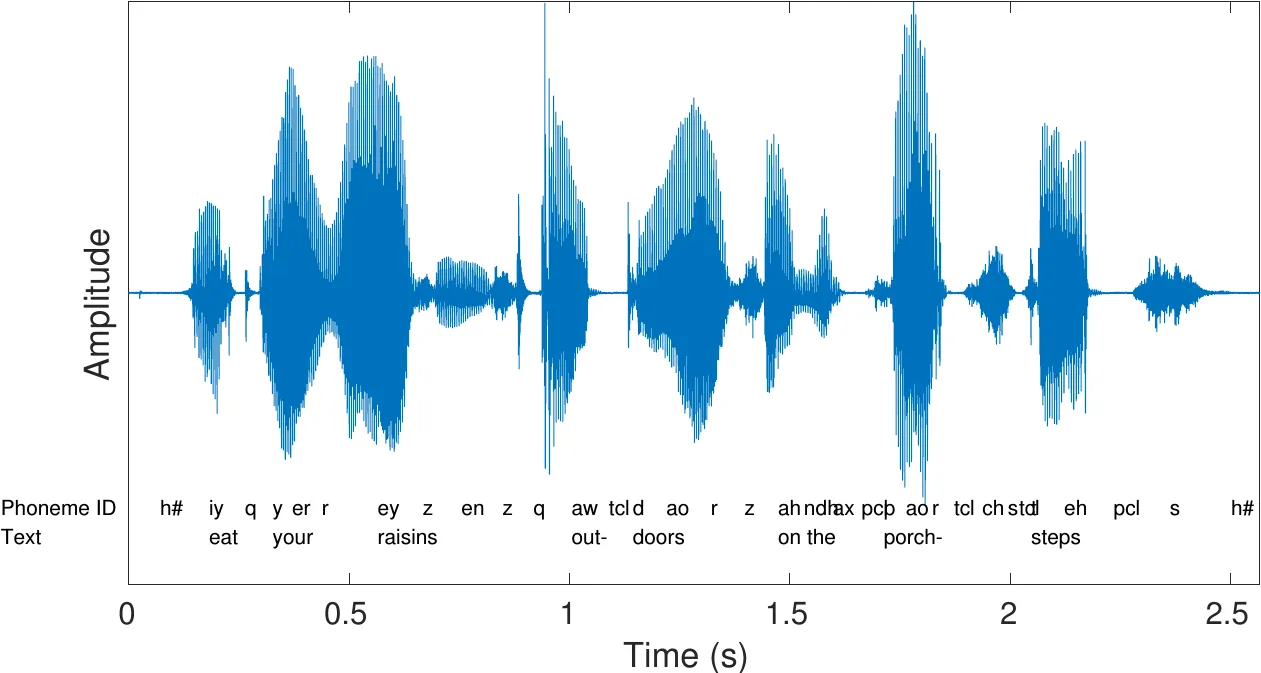
Figure 2. A waveform shows how sound amplitude changes over time. It is the raw shape of audio, but by itself it does not clearly reveal words, phonemes, or frequency structure.
The waveform is useful because it shows the signal over time. But it is also hard to interpret. If we only look at amplitude changing over time, we do not immediately see which frequencies are present or where linguistic units begin and end.
Before a model can use audio, the continuous signal must be digitized. Two basic steps matter here: sampling and quantization.
Sampling decides when we measure the sound wave. A continuous wave has infinitely many points, but a computer needs a finite sequence of values. The sampling rate tells us how many measurements are taken per second. For example, 16 kHz audio means the system records 16,000 samples per second.
Quantization decides how precisely each measurement is stored. Since computers use finite numbers, the continuous amplitude must be mapped into discrete bins. Too few bins make the audio rough and distorted. More bins preserve the original wave more faithfully.
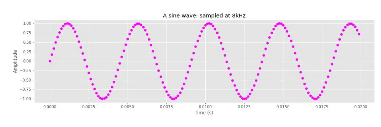
Figure 3. Sampling turns a continuous wave into values over time. Quantization maps those values into discrete levels so the computer can store them.
After this step, speech becomes a sequence of numbers. But this still does not mean the model has a good representation. Raw waveform values are often too low-level. The model still needs a way to reveal the structure inside sound.
From Waveform to Frequency
Speech is not only amplitude over time. Different sounds have different frequency patterns. Vowels, consonants, background noise, and music may occupy different frequency regions. These patterns are not always obvious from the waveform.
This is where the Fourier Transform becomes useful. The idea is to decompose a complex waveform into simpler periodic components at different frequencies. Instead of only asking how the signal changes over time, we also ask which frequencies are present and how strong they are.
Once we represent frequency across time, we get a spectrogram.
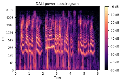
Figure 4. A spectrogram shows sound across time and frequency. Time is usually on the horizontal axis, frequency on the vertical axis, and intensity is shown through brightness or color. Source.
This representation is much more informative than a raw waveform for many speech tasks. It lets us see how energy moves across frequency bands over time. Older ASR systems relied heavily on engineered acoustic features such as spectrograms, mel-spectrograms, and MFCCs.
Modern systems still care about representation, but the method has changed. Instead of forcing humans to design every feature, models increasingly learn representations directly from large audio datasets.
Feature Engineering vs Representation Learning
Earlier speech systems depended on feature engineering. The pipeline was usually carefully designed: extract acoustic features, pass them into a statistical model, then decode the most likely word sequence. This worked for decades, but it required a lot of expert design.
Modern speech systems move toward representation learning. Models such as wav2vec 2.0 and HuBERT learn useful structure from raw or lightly processed audio. Instead of needing a transcript for every audio clip, they can first learn from large amounts of unlabeled speech.
This is especially important because labeled speech data is expensive. Someone has to transcribe the audio, align it, clean it, and check it. For low-resource languages, noisy recordings, or specialized domains, this can become a serious bottleneck.
Self-supervised speech learning tries to reduce that dependence. The model learns general acoustic and linguistic structure first, then adapts to downstream tasks later.
This shift is similar to what happened in NLP. Instead of training a model from scratch for every task, we pretrain on a large amount of data and fine-tune later. In speech, this means the model can learn useful audio representations before it is explicitly trained for ASR, speaker recognition, or translation.
Automatic Speech Recognition
Automatic Speech Recognition, or ASR, is the task of converting speech audio into text.
At first, ASR looks like a simple input-output problem:
audio → transcript
But the hard part is everything in between. Speech is continuous. Words are not separated by clear boundaries. People pronounce the same word differently. They speak at different speeds. They pause, repeat themselves, mumble, laugh, or talk over each other.
There is also ambiguity. “Ice cream” and “I scream” may sound almost identical. A human listener uses context to choose the likely interpretation. A good ASR system must learn to do something similar.
So ASR is not only acoustic pattern matching. It also requires language modeling. The system has to combine what the audio sounds like with what word sequence makes sense.
How ASR Is Evaluated
ASR is usually evaluated using error rate. The most common metric is Word Error Rate, or WER. It compares the predicted transcript against a reference transcript and counts how many word-level edits are needed. These edits can be substitutions, insertions, or deletions.
There is also Character Error Rate, or CER, which works at the character level. If the reference is RELEVANT and the prediction is ELEPHANT, the edit distance is 3 over 8 characters, so the CER is 37.5%.
WER and CER are useful because they are simple and reproducible. But they are not perfect. They measure surface mismatch, not full meaning. A transcript can preserve the intended meaning but still be penalized if the wording, punctuation, or segmentation differs from the reference.
The Evolution of ASR Architectures
ASR has moved from handcrafted statistical systems to large end-to-end models.
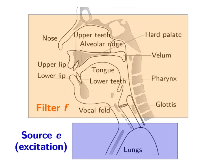
Figure 5. ASR architectures evolved from GMM-HMM pipelines to neural CTC systems, attention-based models, Transformers, and modern speech foundation models. Source.
Early systems often used GMM-HMM pipelines. These systems were efficient and worked well for many years, especially when compute was limited. But they required heavy feature engineering and complex training procedures.
Neural systems changed the field. RNNs helped model sequences, and CTC made it possible to train speech recognizers without exact frame-level labels. Attention-based encoder-decoder models then allowed the model to learn more flexible relationships between audio and output text. Transformers scaled this further by using attention as the main mechanism for sequence modeling.
Today, models such as Whisper-style systems are trained on large, noisy, multilingual audio datasets. This makes them more robust to real-world recordings and more flexible across tasks.
A rough timeline is:
GMM-HMM → RNN + CTC → Attention / Transformers → Foundation Models → Audio LLMs
CTC: Learning Without Exact Timing
One of the key ideas in end-to-end ASR is Connectionist Temporal Classification, or CTC.
The problem CTC solves is alignment. In many speech datasets, we know the transcript, but we do not know exactly when each character or word occurs in the audio. We may know that the audio says “world!”, but not the exact frame where w, o, r, l, d, and ! happen.
CTC allows the model to predict one token per frame while still producing a shorter final transcript. The frame-level prediction can include repeated tokens and blank symbols. Here, ε means a blank symbol, or “no output token at this frame.”
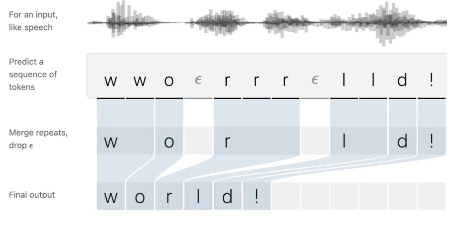
Figure 6. CTC predicts a sequence of frame-level tokens, then merges repeated tokens and removes blank symbols to recover the final transcript. Source.
This is powerful because the training data only needs the audio and the final transcript. CTC handles the hidden alignment problem inside the learning objective, without requiring a human to label exact timing for every character or word.
Attention and Transformer-Based ASR
CTC is useful when we want a monotonic alignment between audio frames and output tokens. But speech recognition also benefits from broader context. A model may need to hear later words before deciding what an earlier ambiguous sound means.
Attention-based models help with this. Instead of processing everything only step by step, attention lets the model look across the input sequence and decide which parts matter when generating each output token.
Transformers push this idea further. They use attention as the central operation, which makes them effective for learning long-range dependencies and scaling to large datasets.
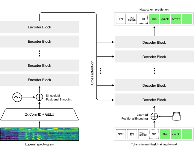
Figure 7. Transformer-based speech models can learn from large multilingual audio datasets and support tasks such as transcription, translation, and language identification. Source.
This is why modern ASR systems are no longer only small acoustic models. They are often large sequence models trained on diverse audio. The gain is not only higher accuracy, but also robustness: different speakers, noisy recordings, accents, and multiple languages become easier to handle.
Streaming ASR
Not every ASR system can wait for the full audio clip. Live captions, voice assistants, and meeting transcription need streaming ASR, where the model processes audio as it arrives.
That is where the tradeoff appears. If the model waits longer, it gets more future context and can make better predictions. If it predicts sooner, the interaction feels faster, but the transcript may be less accurate.
So streaming ASR is therefore not just about recognition quality. It is also about timing. The system has to choose how much delay is acceptable in a real conversation.
From ASR to Audio LLMs
Traditional ASR mostly asks:
What was spoken?
Modern Audio LLM systems ask a broader question:
What does this audio mean, and how should the system respond?
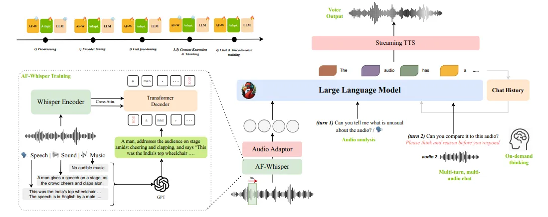
Figure 8. Audio LLMs move beyond transcription. They can use audio as input for reasoning, summarization, question answering, and conversational response. Source.
An Audio LLM does more than turn speech into text. It can summarize a meeting, answer questions about a recording, pick up on tone, or reason about sound events. In that sense, audio is no longer just a preprocessing step before the “real” model starts — it becomes something the model can actually think with.
That difference shows up in the output. A traditional ASR system might simply say, “The meeting starts at 3 PM.” An audio assistant, on the other hand, could infer that the speaker is confirming a schedule change and that the next step is to notify the team. One system transcribes; the other interprets speech in context.
Speech Translation
Speech Translation converts speech in one language into another language. The input may be English speech, and the output may be Vietnamese subtitles or a Vietnamese spoken response.
There are two common designs: cascaded systems and direct end-to-end systems.

Figure 9. Speech translation can be built as a cascaded pipeline or as a more direct model that maps source speech to translated text or speech. Source.
A cascaded system breaks the problem into modules:
ASR → Machine Translation → TTS
First, the source speech is transcribed. Then the transcript is translated into another language. If speech output is needed, a text-to-speech model turns the translation back into audio.
This setup is useful because each part can be improved on its own, and it is easier to debug. If the final result is wrong, we can check whether the problem came from transcription, translation, or speech synthesis.
The downside is that errors can build up. If ASR gets something wrong, the translation model starts from the wrong text. And when speech has to pass through text in the middle, some tone, emotion, pauses, and prosody can get lost.
Direct speech translation tries to avoid some of that by mapping speech straight into translated text or speech. That can lower latency and preserve more of the original signal, but it is harder to train because parallel speech-translation data is expensive and limited.
Evaluating Speech Translation
Speech translation is usually evaluated by comparing the model’s output with a human reference translation. Some metrics focus on surface form. BLEU and ROUGE check for overlapping words or phrases, so they’re quick and easy to compute, but they can miss valid paraphrases.
Other metrics focus more on meaning. BERTScore and COMET try to measure whether the translation keeps the same meaning and sounds fluent. They usually line up better with human judgment, though they take more computation and are harder to interpret.
That’s why evaluation in translation is tricky: matching words is not the same as preserving meaning, naturalness, or tone.
Modern Speech Translation Systems
Modern speech translation is moving toward unified models. Instead of building one separate system for transcription, one for translation, and one for speech synthesis, newer models try to support many directions inside a single framework.
This includes speech-to-text, speech-to-speech, text-to-speech, and text-to-text. Whisper-style models show how a large multilingual speech model can support robust transcription and translation. More recent unified speech systems push further toward many-to-many speech and text translation.
The trend is that speech systems are becoming less like isolated pipelines and more like multimodal foundation models. They do not only hear speech. They connect speech with text, translation, dialogue, and reasoning.
Takeaways
Speech processing begins with sound, but it does not end with transcription.
The first challenge is representation. A computer has to turn continuous audio into machine-readable signals through sampling, quantization, and feature extraction or learned representations.
The second challenge is meaning. Speech contains words, but also speaker identity, accent, emotion, context, environment, and interaction.
The third challenge is system design. ASR, speech enhancement, speaker analysis, TTS, and speech translation can be built as separate modules or combined into larger end-to-end systems.
The most interesting direction is that speech AI is moving from narrow transcription systems toward models that can listen, understand, translate, reason, and respond.
You can play around with the audio things here: meralion.org/playground.